Ren is with Department of Biomedical Engineering, National University of Singapore, Singapore and NUS (Suzhou) Research Institute (NUSRI), China (e-mail: ren@nus.edu.sg).
Color versions of one or more of the figures in this paper are available online at http://ieeexplore.ieee.org.
Digital Object Identifier 10.1109/JSEN.2015.2456181
INTRODUCTION
F
LEXIBLE robots such as wire-driven robots or continuum robots have been well studied. Researchers have been inspired with the incredible capabilities for locomotion, manipulation, and dexterity exhibited by snakes, elephants’ trunks, tongues, and octopus tentacles and therefore work toward recreating their capabilities in electromechanical devices [1]. Compared with traditional discrete rigid robots, flexible robots are compliant and suitable for the confined environments, such as the minimally invasive
surgery (MIS).
As a typical MIS, transoral surgery brings to patients significant benefits such as decreased intraoperative blood loss, less post-operative complication morbidity, shorter length of hospitalization and recovery period [2]. Generally, there are two types of flexible robots suitable for transoral surgery. One is the tendon/wire/cable-driven manipulators [3] and the other is the concentric tube robots [4], [5]. The tendon/wire/cable-driven manipulators compose of a flexible backbone and a number of tendons/wires/cables [6]. The flexible backbone is either serpentine backbone similar to the snake spine column or continuum backbone which mimics the elephant trunk. The backbone can be deformed by controlling the tendon/wire/cable motion, therefore to realize the pose control of the distal end.
The drawback of the flexible robot is that the joints’ rotations cannot be controlled independently, therefore the backbone deformation cannot be controlled at will and the joints rotations are unknown. As a result, the real time positional and shape information cannot be well estimated, especially when there is external load on the end tip or external force working on the robot. The pose and shape information are important for the operation process due to the following reasons
The robot may interact with tissues during the surgery. Tissues will affect the position and shape of the robot, and meanwhile the robot may damage the tissues. Therefore, positional and shape information of the robot need to be estimated in real time to reduce the unexpected injury on the tissues during the surgery.
Feedback control is required during the operation. In order to perform accurate maneuvering, real time positional and shape information are necessary to be provided as feedback to the controller.
1530-437X © 2015 IEEE. Personal use is permitted, but republication/redistribution requires IEEE permission.
See http://www.ieee.org/publications_standards/publications/rights/index.html for more information.
Kinematic based model [1], [7]–[11] is the most used method for shape detection. The backbone deformation is estimated by kinematic modeling with some assumptions, such as the piecewise constant curvature assumption [9]. This method can only estimate the shape of the backbone without payload. A more accurate shape estimation is to use the Cosserat Rod Theory [10] and incorporate with the statics model. Xu and Simaan [8] proposed a method using ellip- tical integrals to achieve the shape restoration with a known extern load. Trivedi et al. [12] presents a new approach for modeling soft robotic manipulators that incorporates the effect of material nonlinearities and distributed weight and payload. The model is geometrically exact for the large curvature, shear, torsion, and extension that often occur in these manipulators. In [7], a model based on a Rayleigh-Ritz formulation is proposed. By using the transversal tip force and distributed load as inputs, the needle deflection can be predicted. The drawback of these model based methods is that, the forces applied to the backbone needs be known in prior. In a real application, these forces is usually unknown and thus these model based shape estimation methods are of limited use.
Sensor based technologies have also been studied and used for tracking and shape reconstruction. Medical image based methods are often used, such as Ultrasound [13], [14] and Magnetic Resonance Imaging (MRI) [15]. Another popular technology that has been well studied is Fiber Bragg Grating (FBG) [16], [17] based method. Usually, a number of FBG sensors are mounted in the robot. The FBG sensors can measure the axial strain of the placed position, which enables the computation of the needle curvature. The three-dimensional (3-D) robot shape can then be reconstructed from the curvature. Electromagnetic tracking (EMT) method is also reported to detect the collision detection and estimate the contacted location along multi-segment continuum robots [18].
−
×
In this paper, we proposed a general shape reconstruction method for the flexible robots with multiple bending sections, such as wire-driven flexible robots or concentric tube robots. The curvatures of each bending section are varying. The proposed method is based on the electromagnetic tracking and fitting of a number of Bézier curves. Compared to the image or optic based tracking method, the EMT method does not have the line-of-sight problem [19]–[22]. Therefore, EMT method functions properly for the tracking applications in MIS. For a N -section robot, N/2 electromagnetic sensors will be mounted at the tail of the (N 2k)th section, where
≤
0 k < n/2. Therefore, by utilizing the positional and
directional information of the sensors, each section can be reconstructed based on a quadratic Bézier curve. Compared to the image based method, this method is easy to setup; compared to the FBG based method, curvature information is not used and fewer sensors are needed in the proposed method.
The primary contributions of our work are summarized as follows:
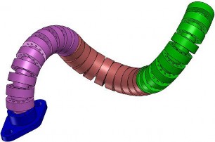
Fig. 1. Multi-section wire-driven flexible robot. The shown robot has three bending sections. Each section can be controlled independently to deform as an arc with different curvatures.
N
×
positional and directional information of a few specific joints on the robot.

For a N -section robot, only 2 electromagnetic sensors are needed. Very few modifications will be made on the
robot.
Compared with the MRI, FBG and kinematic based method, the proposed method is easy to set up and meanwhile has a good accuracy.
No prior curvature information is needed for the shape reconstruction.
The organization of this paper is as follows. In Section II, the structure and mathematic model of the multi-section wire-driven robot will be presented. In Section III, the shape reconstruction method will be presented in detail. In Section IV, the simulation experiment results will be shown. The experimental results will be shown in Section V and conclusions will be made in Section VI.
MULTI-SECTION FLEXIBLE ROBOT
Background
The wire-driven flexible robot mimics the animal backbone musculoskeletal structure [3], [23]. As shown in Fig. 1, the robot contains three bending sections. Each section can be controlled independently to deform as an arc with different curvatures. A pair of wires goes through the guiding holes and the deformation is made by the wires. The joints’ rotations are controlled by the wires and the backbone.
The forward kinematic model of the multi-section tendon-driven robot is shown in the following part.
Kinematic Model
=
As shown in Fig. 2, for the i -th section (i 1, 2, ...M), the backbone length is Li , the bending angle is i , the bending direction is i , the twist ξi is (ωi ,υi ) [24] and the number of joints is Ni . Based on the constant curvature assumption and the product of the exponential expression, the transformation
R
p
1
matrix gi−1,i of the section is as follows,
A general reconstruction method for multiple bending sections with different curvatures is proposed based on Bézier curve fitting method. This method only needs the
gi−1,i(ωi, υi) = eξˆi i =
i−01,i i
(1)
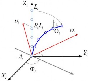
Fig. 2. Kinematic model for the i-th section. The backbone length is Li , the bending direction is i , the total bending angle is i and the twist ξi is (ωi , υi ). Ai and Bi are defined in (3).
⎪⎨
where Ri−1, j is the rotation matrix and pi is the translation vector. The twist coordinates ξi (ωi, υi ) are as follows,
When the backbone deforms, the shape is smooth and neighboring joints’ rotations are similar. Theoretically, each section will be an arc from a circle after deformation. Therefore, the piecewise constant curvature assumption is available for the shape reconstruction. However, the curvature information is hard to estimate. In the following part, the proposed shape reconstruction method will be introduced, which is not based on the kinematic model and no curvature information is needed.
CURVE SHAPE SENSING METHOD
The proposed method is based on curve fitting of the quadratic Bézier curve. First the Bézier curve will be intro- duced and then the reconstruction method will be shown.
Bézier Curve
A Bézier curve is a parametric curve frequently used in computer graphics and related fields.
The formula for the Bézier curve of order n can be expressed explicitly as follows,
n
⎧ω
i
⎪⎩
υi
where
= − sin( ) cos( ) 0 T
i
i
T
= − Ai cos( i) − Ai sin( i) Bi Li
B(t) = bi,n(t)Pi (5)
(2)
i=0
∈ [ ]
i
where t 0, 1 . P0 is the start point of the curve, Pn is the end point and Pi (0 < i < n) is the control point. bi,n is defined as follows,

⎧⎪Ai = Li (Ni − 1)
2Ni
⎪ 1 1
i
i


bi,n =
n ti (1 − t)(n−i) (6)
⎨Bi =
⎪
2Ni
ωˆ
i
cot
υ
2Ni −
2 cot 2
(3)
The Bézier curve that used in this paper is the quadratic Bézier curve. As shown in Fig. 3, several quadratic Bézier curves combine together to model the multi-section flexible
⎪⎩ξˆi =
i ∈ R4×4
robot. Each section will be modeled with a quadratic Bézier
0 0
ˆ
among the above equations, ωi is the skew matrix associated with ωi . The overall transformation g0, M can be established as shown in the following equation based on the chain rule.
M
g0,M = gi−1, j (ωi , υi) (4)
i=1
The parameters used in the above equations are defined as
curve. Assume there are N sections, for the k-th section. P2k−2 is the start point, P2k is the end point and P2k−1 is the control point. The curve starts at P2k−2 and arrives at P2k coming from the direction of P2k−1. Hk is the unit direction vector of the curve at position Pk. P2k 1 is the control point. The
−
explicit form of the k-th curve is
Bk(t) = (1 − t)2P2k−2 + 2(1 − t)tP2k−1 + t2P2k (7)
where 0 ≤ t ≤ 1, 1 ≤ k ≤ N .
follows:
⎪
⎧eξˆθ
⎪⎨
⎪
eωˆ θ (I − eωˆ θ)ωˆ + ωωT θ υ
0 1
0 −ω3
ω2
⎤
=
B-spline curves are often used to fit a curve. Compared to the B-spline curves, the Bézier curve has the following advantages: 1) the positional information of the electromag- netic sensors can be directly used as the start point and end
point of the Bézier curve; 2) the directional information of the sensors can be directly used to express the control points
⎪
⎡
ωˆ = ⎢⎣
⎩
⎪
ω3 0 −ω1
−ω2 ω1 0
with the unknown parameters. The above advantages make the Bézier curve a very good choice for shape reconstruction for EMT based shape sensing. Besides, there is no other known
⎥⎦
eωˆ θ = I + ωˆ sin θ + ωˆ 2(1 − cos(θ))
where ω1, ω2, ω3 are the three components of ωˆ .
position or direction information of the points between the start point and end point, therefore B-spline curves may not be a good choice for this research.
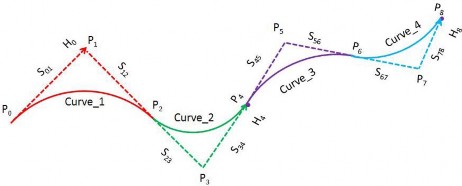
Fig. 3. Quadratic Bézier curves combine together for a four sections flexible robot. Two sensors are mounted in the robot, one is at the tail of the second section and the other is at the tail of the fourth section. Each section is reconstructed with a quadratic Bézier curve. With the known parameters P0, H0, P4, H4, P8 and H8, the four curves can be solved.
Setup for the Shape Reconstruction Method
Before introducing the reconstruction method, some properties will be drawn.
= =
=
= || || = || ||
= || ||
As shown in Fig. 3, define Si, j PiPj , for example, S01 P0P1 , S12 P1P2 . According to the multi- section robot model, each section is an arc from a circle, therefore for the k-th section, S2k−2,2k−1 S2k−1,2k. For example, as shown in Fig. 3, S01 S12, S23 S34,
= =
S45 S56, S67 S78,
+ − +
For section k and section k 1, P2k 1, P2k and P2k 1 are in the same line. For example, as shown in Fig. 3, P1, P2 and P3 are in the same line; P3, P4 and P5 are in the same line;
Although the curves in Fig. 3 are drawn in the same plane, it is not pre-requisite. The relationships mentioned above and below are still valid when the curves are in the different planes. The method is the same in this case;
In the real flexible robot device, P0 is in a fixed position with a fixed direction;
The known parameters from the structure of the robot
Reconstruction Method for the Group With One Quadratic Bézire Curve
When section number N is odd, the reconstruction method for the first section with one quadratic Bézier curve will be proceeded. In this case, according to the sensor position that mentioned in the above section, a sensor will be fixed at the end of the first section.
= + = || ||
As shown in Fig. 3, the sensor will be mounted at P2. The known parameters for the first section, here denoted as curve1, are P0, H0, P2 and curve length L1. According to (7), the parameter that needs to be solved is P1. It can be seen that P1 P0 S01H0, where S01 P0P1 . Therefore, the only unknown parameter is S01, and the equation for solving the parameter will be
L1 − Ls1 = 0 (8)
where Ls1 is the estimated length of the curve, it can be estimated as follows,
is the length information Li
of each section.
n
L = ||B
i − B ( i − 1 )|| (9)


The electromagnetic sensor will be mounted on tail of the (N − 2k)th section, where N is the total section number

s1
i=1
1( n ) 1 n
2
≤
and 0 k < N . In another way, the sensors will be
−
placed at positions P2(N 2k). As shown in Fig. 3, there are 4 sections, therefore the sensors will be placed at the end of the 2nd and 4th sections, which are denoted as P4 and P8.
where n is the number of points that used to estimate the curve length on the Bézier curve B1. In this paper, we set n equal to the joint number of the robot. Therefor, each joint in the
robot will have a corresponding point on the Bézier curve.

Therefore, only × N sensors are needed for the shape
2
B is as follows,
reconstruction. 1

2
×
The reconstruction method will first divide the sections into N groups. If the section number N is even, the reconstruction method will be carried out from the first group. For each group, it contains two sections, the parameters of two quadratic Bézier curves will be solved based on the curve length information; if N is odd, the reconstruction method will be proceeded from the second group. For each group, it contains two sections, the parameters of two quadratic Bézier curves will be solved based on the curve length information. The first group contains only one section and will be solved with one quadratic Bézier curve. The reconstruction method for the two different groups will be introduced in the following part.
B1(t) = (1 − t)2P0 + 2(1 − t)tP1 + t2P2 (10)
Therefore, S01 can be solved with (8).
Reconstruction Method for the Group With Two Quadratic Bézire Curves
For the groups that contain two sections, a sensor is mounted on the starting position of the first section and the other sensor is mounted at the end position of the second section. As shown in Fig. 3, take section 3 and section 4 for example. This group contains two quadratic Bézier curves. The sensors are mounted
⎧⎪⎨
at P4 and P8. The following equations can be obtained.
P5 = P4 + S45H4
P7 = P8 − S78H8
(11)


||P1P3||
S45 + S78
⎪⎩P6 = P5 + S56 P3 − P1 = P5 + S45 (P3 − P1)
where P4, P5 and P6 are the start point, control point and end point of Curve3. P6 is also the start point of Curve4. P7 and P8 are control point and end point of Curve4. H4 and H8 are the tangent vectors of the curve at point P4 and P8. The two Bézier curves can then be presented as follows.
B3(t) = (1 − t)2P4 + 2(1 − t)tP5 + t2P6
B4(t) = (1 − t)2P6 − 2(1 − t)tP7 + t2P8
(12)
where B3 is for Curve3 and B4 is for Curve4. Define the unknown parameters as (S45, S78). Based on the above information, two equations can be established.
L3 = Ls3 (13)
L4 = Ls4
where Ls3 and Ls4 are the estimated lengths of Bézier curve3 and Bézier curve4. L3 and L4 are the lengths of the sections from flexible robot. Therefore, S45 and S78 can be solved.
General Equations
Generally, for the group that contains k-th section and
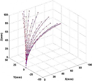
Fig. 4. Simulation results of curves with one section. In the experiment, 12 curves are generated based on (4) with one circle. 13 joints have been used in the experiment to generate the curve. Blue stars represent the ground truth generated by numerical method and red lines represent the reconstruction results.
where Lsk can be estimated with the following equation.


nk
nk
nk
Lsk = ||Bk( i ) − Bk( i − 1 )|| (18)
i=1
+ +
(k + 1)-th section, the sensors are mounted on the starting position of the k-th section (P2k−2) and the ending position of the (k+1)-th section (P2k+2). Therefore, the known parameters are P2k−2, H2k−2, P2k+2, H2k+2, Lk and L(k+1), where H2k−2 and H2k+2 are the tangent vectors of the curve at point P2k−2 and P2k+2, Lk and L(k+1) are the curve length from the robot. The parameters to be solved are S2k−2,2k−1 and S2k 1,2k 2. The relationships between these parameters are
shown as follows,
⎧⎪⎨P2k−1 = P2k−2 + S2k−2,2k−1H2k−2
where nk is the number of points that used to estimate the curve length for the k-th Bézier curve. In this paper, we set nk equal to the joint number of the k-th section of the robot. Therefore, each joint in the robot will have a corresponding point on the Bézier curve.
SIMULATION AND DISCUSSION
Simulation
In this section, we carry out the simulation experiments to show the performance of the curve reconstruction
⎪
P2k+1 = P2k+2 − S2k+1,2k+2H2k+2
⎩P2k = P2k−1 + Sk(P2k+1 − P2k−1)
(14)
method. The experimental data is generated based on (4). The curve reconstruction algorithm is then used to fit the numerical data based on quadratic Bézier curves and the
+
+ − +
where P2k is the ending position of k-th section and the starting position of the (k 1)-th section. P2k 1 and P2k 1 are the control points of the k-th and (k 1)-th section. Sk is defined as follows,
S2k−2,2k−1

Levenberg-Marquardt (LM) algorithm.
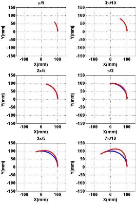
In the experiment, four groups of multi-section curves are generated based on (4) with different number of sections. The results can be seen from Fig. 4 to Fig. 7.
Fig. 4 shows the experimental results of the one section
,
Sk = S2k−2 2k−1
+ S2k+1,2k+2
(15)
curve reconstruction, where the blue line represents the ground truth generated by numerical method and the red line repre-
The equations of the two Bézier curves are sents the reconstruction result. Fig. 5 shows the experimental
Bk(t) = (1 − t)2P
2k−2
+ 2(1 − t)tP
2k−1
+ t2P2k
(16)
results of robot shape reconstruction with two sections. Fig. 6 shows the three-section flexible robot shape reconstruction and
Bk+1(t) = (1 − t)2P2k + 2(1 − t)tP2k+1 + t2P2k+2
− − + +
Therefore, with the length information Lk and L(k+1), S2k 2,2k 1 and S2k 1,2k 2 can be solved. The equations are as follows,
Fig. 7 shows the experimental results of curve reconstruction with four sections. In these figures, different colors are used to represent the reconstruction results of different sections.
Error Evaluation
Lk = Lsk
Lk+1 = Ls(k+1)
(17)
In this paper we use the distance error of the crossing points to evaluate the performance of the reconstruction method.
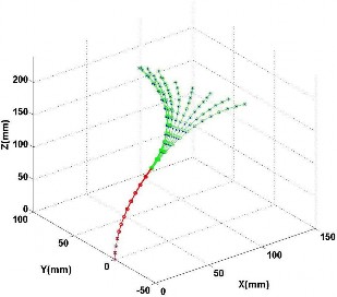
Fig. 5. Simulation results of curves with two sections. In the experiment, 12 curves are generated based on (4) with one circle. 25 joints have been used in the experiment to generate the curve. Blue points and lines represent the ground truth generated by numerical method, red circles and lines represent the reconstruction results for the first section and green lines are for the results of the second section.
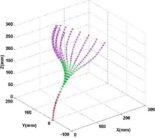
Fig. 6. Simulation results of curves with three sections. In the experiment, 12 curves are generated based on (4) with one circle. 37 joints have been used in the experiment to generate the curve. Blue points and lines represent the ground truth generated by numerical method. Red, green and purple circles and lines represent the reconstruction results of the first section, second section and third section, respectively.
In the numerical simulation, for the multi-section curves, the length of each section is 120mm.
The crossing joint means the joint between two sections and without sensor mounted. As shown in Fig. 8, for a two-section curve, the crossing point used to perform the error evaluation is P2; for a three-section curve, the crossing point is P4; for a four-section curve, the crossing points are P2 and P6. Fig. 8 shows the results of these points. The average distance error of these points are 0.56mm.
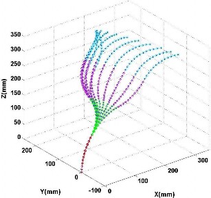
Fig. 7. Simulation results of curves with four sections. In the experiment, 12 curves are generated based on (4) with one circle. 49 joints have been used in the experiment to generate the curve. Blue points and lines represent the ground truth generated by numerical method. Red, green, purple and cyan lines and circles represent each section, respectively.
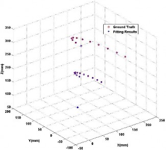
Fig. 8. Simulation results for the crossing points.
Discussion
Although the simulation results show the effectiveness of the method, there are still two drawbacks:
The method is based on quadratic Bézier curves. For a bending section, if the radian of the curve is more than π/2, the method will be invalid, which can be seen in Fig. 9. The results get worse after the radian surpass- ing π/2. Therefore, a high order Bézier curve is needed for the reconstruction. For a section whose starting and ending positional and directional information are known, a three order Bézier curve can be estimated to perform the reconstruction if the radian is less than π [25];


2
Fig. 9. Reconstruction result for a circle arc using quadratic Bézier curve. The results get worse after the radian surpassing π .
The quadratic Bézier curve is determined by three points, the starting point, the ending point and the control point. It gives the result that the points on the curve should in the same plane. Therefore, if a bending section is deformed to different planes, the method will lose efficacy for this section.
EXPERIMENTS
= =
In order to verify the performance of the proposed method, an experimental platform has been built. As shown in Fig. 10(a), it includes two part, a wire-driven flexible robot with two sections and an electromagnetic tracking system. The robot has two sections, each section can be controlled independently. The EMT system is 3D Guidance trakSTAR (Northern Digital Inc.). TrakSTAR is a high-accuracy elec- tromagnetic tracker designed for short-range motion tracking applications. It employs the pulsed direct current (DC) tech- nology to track the position and orientation of multiple sensors within the operating range of the transmitter. Sensor data is reported serially to a host computer via a USB or RS232 interface. It has three parts, the electronics unit (it supports up to 4 sensors), the transmitter (mid-range model, its translation range is 46cm with model 180 sensor) and the 6 degrees- of-freedom (DOF) sensors (Model 180 6DOF sensor, sensor OD 1.5mm, sensor length 7.7mm). The pulsed DC signal is transmitted by the transmitter and received by the sensors. With these sensing signals, the system can output the position and orientation (azimuth, elevation and roll) information of each sensor. The static accuracy of this system are 1.4mm
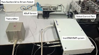

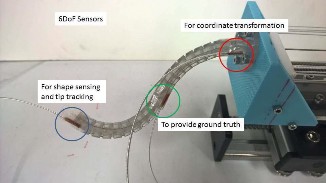

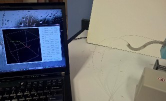

Fig. 10. Experimental Platform. (a) The platform includes two part, the wire-driven flexible robot and the electromagnetic tracking system. The robot has two sections, each section can be controlled independently. The EMT system has three parts, the control unit, the transmitter and the 6DoF sensors.
(b) Three sensors have been mounted on the robot. The one that mounted on the distal end of the robot is the working sensor, its position and orientation information is used to perform the tip tracking and shape sensing. The sensor that mounted on the base of the robot is to provide transformation information between EMT coordinate system and robot’s coordinate system. With this sensor fixed, there is no need for calibration between these two system. The sensor that mounted on the cross joint of the robot is to be the reference. It provides the position of the cross joint, which can be used as the ground truth for the shape sensing method. (c) The shape reconstruction algorithm has been implemented with C++. Real time display interface is made by Microsoft Visual Studio 2010 and OpenGL.
root-mean-square (RMS) of position and 0.5 degree RMS of orientation [26].
As shown in Fig. 10(b), three sensors have been mounted on the robot. The one that mounted on the distal end of the robot
is the working sensor, its position and orientation information is used to perform the tip tracking and shape sensing. The sensor that mounted on the cross joint of the robot is to serve as the reference. It provides the position of the cross joint and therefore the ground truth for the evaluation of the performance of the shape sensing method can be obtained. The sensor that mounted on the base of the robot is to provide transformation information between EMT coordinate system and robot’s coordinate system. With this sensor fixed, there is no need for calibration between these two system. The coordinate transform method is shown in the following part.
Use R, E , S0, S to represent the coordinate systems of robot, EMT system, base sensor and tracking sensor. As the base sensor is fixed on the robot, therefore the transformation
S
matrix TR
0
that between base sensor and robot is known.
Therefore, the position and direction of tracking sensor in robot coordinate system is
⎛ xs ms ⎞
⎛ 0 1 ⎞
⎝ ⎠
⎝ ⎠
zs ps
1 0
S
0
E
E
0 0
1 0
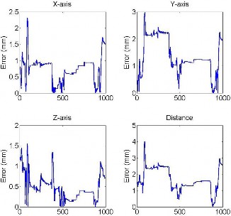
Fig. 11. Experimental results of the position error of the reference sensor that mounted on the cross joint of the robot.
⎜ ys ns ⎟ = TR (TS0 )−1TS ⎜ 0 0 ⎟
(19)
where (xs, ys, zs)T is the position and (ms, ns, ps)T is the unit direction vector of X-axis of the tracking sensor in robot coordinate system. TS0 is the transformation matrix between
CONCLUSION