INTRODUCTION
UTOMATED monitoring-diagnostics of the robotic sys- tem play a crucial role for the use of robotic manipulators
Manuscript received May 15, 2015; revised November 20, 2015 and
February 16, 2016; accepted April 6, 2016. This work was supported in part by the ASTAR TSRP Project under Grant R-261-506-008-305 and Grant R-261-506-007-305, and in part by the Human–Robot Collaborative Systems in Industrial Unstructured Environments: Sensing and Perception and Office of Naval Research Global under Grant ONRG-NICOP-N62909-15-1-2029. This paper was recommended by Associate Editor P. Shi. (Corresponding author: Hongliang Ren.)
S. S. Ge is with the Department of Electrical and Computer Engineering and Social Robotics Laboratory, National University of Singapore, Singapore 117580 (e-mail: samge@nus.edu.sg).
H. Ren is with the Department of Biomedical Engineering and Advanced Robotic Centre, National University of Singapore, Singapore 117580 (e-mail: ren@nus.edu.sg).
Color versions of one or more of the figures in this paper are available online at http://ieeexplore.ieee.org.
Digital Object Identifier 10.1109/TCYB.2016.2555307
as parts of autonomous system. Various fault diagnosis (FD) approaches for robotic systems have been studied in the litera- ture based on the model-based methods [1]–[3]. Using intelli- gent learning techniques such as neural network (NN) or fuzzy logic, robust FDs have been proposed [4]–[10]. However, the disadvantage of the uses of learning techniques is that they provide a difficulty in implementation and huge computation due to the complication in training of neural weights or fuzzy rules. Due to its inherent robustness to system uncertainties and external disturbances, sliding mode observer has been used in the design of fault diagnostic observers [11]–[15]. Although this technique is simple in design and has a fast convergence; however, the design system requires a prior knowledge of bounded faults, which could be, from a practical point of view, hard to acquire. In robotic system, it is well known that faults usually occur at unknown time and with unknown mag- nitude. To relax the requirement of bounded faults of sliding mode observer, neural sliding mode observers, which combine the NN and the sliding mode observers, have been developed in our previous studies [16], [17]. However, these approaches still contain the intelligent learning technique; it may meet, as aforementioned, a difficulty in real implementation. Time delay estimation (TDE) technique developed in [18] and [19] is a simple but robust technique to approximate a nonlinear function without prior knowledge on bounded unknown input by using time delay information. This technique has been suc- cessfully used to approximate the unknown dynamic model of robot manipulators [20]–[22]. However, to the best of the author’s knowledge, there is no study in literature on the use of TDE to carry out robust FD.
After a fault is diagnosed, fault tolerant control (FTC) should be employed to compensate for the effects of the faults in the system so that the system can continue to reliably work in the presence of faults [23]. In literature, the approaches of FTC can be divided into two categories: 1) active and
2) passive [24]. In passive FTC (PFTC) systems, the partial knowledge of the fault is assumed to be known in advance and the effects of the fault are considered as the effects of an addi- tional disturbance. Then, the robust control scheme is designed to compensate for the fault without the need to detect the presence of a fault [25]–[28]. In contrast, active FTC (AFTC) is designed based on the online estimated fault information, which is obtained by using FD observer [3]–[9], [29]–[33].
2168-2267 ×c 2016 IEEE. Personal use is permitted, but republication/redistribution requires IEEE permission.
See http://www.ieee.org/publications_standards/publications/rights/index.html for more information.
2 IEEE TRANSACTIONS ON CYBERNETICS
In comparison with the PFTC, the AFTC provides better per- formance when the fault information is estimated correctly, and hence, is more desirable for practical applications.
Although many FTC schemes have been developed in the literature for various linear and nonlinear systems, to the best knowledge of the authors, there have been only minor FTC investigations for robotic systems with providing fast finite time convergence. In fact, most of the devel- oped FTC schemes for robot manipulators are designed based on modification of the nominal computed torque controller (CTC) [4]–[8], [16], [17]. However, the use of CTC does not robust to the uncertainties and faults, which may result in poor performance. Many advanced control approaches have been proposed to increase the performance of the robot system for normal operation, such as adaptive control [34], [35], fuzzy control [36], [37],
NN control [38], [39], optimal control [40], sliding mode
control (SMC) [41], [42], etc.
Compared to other methods, SMC has attractive advantages of robustness to uncertainties and disturbances and low sensi- tivity to the system parameter variations [11], [43]. This tech- nique has been used for the design of FTC system [44], [45]. However, because the design is based on a linear sur- face, the uses of traditional SMC scheme do not converge to the equilibrium point in finite time. Recently, terminal SMC (TSMC) methods [46], [47], which use nonlinear sliding surfaces instead of linear surfaces, have been developed. By suitably designing the parameters, the TSMC assures the sys- tem states to reach the equilibrium point in finite time, and also offers some superior properties such as rapid response, robust- ness, and higher precision. However, the initial TSMC has two disadvantages: the first is that it has slower convergence to the equilibrium than the traditional linear SMC when the system state is far away from the equilibrium and the second is the singularity problem. To overcome the first disadvantage of the traditional TSM, fast terminal sliding mode (FTSM) control has been developed [48], [49]; however, these approaches still have a singular problem. In order to eliminate the singular problem, nonsingular TSMC (NTSMC) [50]–[53] and nonsin- gular fast TSMC (NFTSMC) [54]–[57] have been proposed. Compared to the NTSMC, the NFTSMC has the same prop- erty but provides a faster state convergence. However, both SMC and TSMC techniques have a drawback that they pro- duce the high-frequency oscillations of the controller output, known as chattering. In practical implementations, chattering is undesirable because it may excite unmodeled high frequency plant dynamics resulting in unforeseen instabilities. To remove the chattering, several solutions have been proposed. The first is to use the boundary layer approach that replaces the sign function by saturation [56] or sigmoid function [58]. However, this approach produces large steady state errors due to the bound of the saturation function. A second solution is to design of a continuous control law [49], [57]. However, this tech- nique implies deterioration accuracy and/or robustness. A third solution proposed to decrease the chattering is the high-order sliding mode (HOSM) technique [59]–[66]. The basic idea of the HOSM is to move the discontinuous control action to the higher derivatives of the control, and thus the control signal
become continuous. The major advantage of the HOSM when compared to other chattering elimination methods is that it not only eliminates the chattering but also increases the accuracy. In light of the remarkable benefits and limitations, this paper investigates a finite time AFTC scheme for uncertain robot manipulator based on TDE and NFTSMC combined with an HOSM control technique so as to accommodate both the uncer- tainties and faults. To highlight the benefits of the proposed AFTC, the PFTC based on NFTSMC is first presented; and its benefits and limitations are analyzed. Then, based on the limita- tions, the AFTC based on NFTSMC and TDE is then proposed. In this scheme, TDE is proposed as a robust FD scheme to approximate the fault information; the obtained fault informa- tion is used to detect, isolate, and accommodate the effects of faults. Then, NFTSMC is used to compensate for the TDE error and stabilize the control system. Finally, a super-twisting (STW)
HOSM algorithm is employed to eliminate the chattering. Comparing to the existing FTC approaches for robot manip-
ulators, the contribution of this paper can be marked as the following significant points.
Unlike the intelligent learning techniques or sliding mode observer, TDE-based FD scheme is proposed for the first time.
A novel fast finite time AFTC scheme is proposed based on the combining of TDE-based FD, NFTSMC and HOSM controllers.
The proposed FTC system considers and compensates for the effects of both the uncertainty and fault in both healthy and fault operations.
The proposed FTC scheme possess several advantages over other state-of-the-art approaches such as higher pre- cision, robustness, no singularity, less chattering, fast finite time convergence, and no need for prior knowledge of bounded faults.
The rest of this paper is organized as follows. Section II formulates the problem and gives preliminaries. Sections III and IV introduce the design of proposed PFTC based on NFTSMC and proposed AFTC based on NFTSMC and TDE, respectively. The simulation results for a PUMA560 robot are given in Section V so as to verify the effectiveness of the proposed algorithms. Finally, the conclusions are given in Section VI.
PROBLEM STATEMENT AND PRELIMINARIES
Problem Statement
Consider the robot dynamics described by [16], [17]
q¨ = M−1(q)(τ − Vm(q, q˙)q˙ − F(q˙) − G(q) − τd)
+ γ t − Tf φ(q, q˙,τ ) (1)
− ∈
˙ ∈
∈
∈
˙ ∈
˙ ∈
∈ ∈
where q n is the position vector, M(q) nxn denotes the inertia matrix, Vm(q, q) n expresses the Coriolis and centripetal forces, F(q) n represents the friction matrix, τd is a load disturbance matrix, G(q) n is the gravity vector, and τ n is the vector of control torque produced by the actuators. The term φ(q, q,τ ) n denotes the fault vector, γ (t Tf ) n expresses the time profile of the faults, and Tf is the time of occurrence of the faults.
VAN et al.: FINITE TIME FTC FOR ROBOT MANIPULATORS USING TDE AND CONTINUOUS NFTSMC 3
The robot dynamics (1) have the following standard prop- erties. The inertia matrix M(q) is symmetric positive defi- nite, and
The sign function is defined as
⎧⎨ 1 if x > 0
=
0 < λm{M(q)}≤ M ≤ λM{M(q)}≤ χ, χ > 0 (2)
sign(x) =
0 if x 0
⎩ −1 if x < 0.
{ } { }
where λM M and λm M are the maximum and minimum eigenvalues of matrix M.
The time profile of the faults, γ (·), has the following form:
The power of error vectors are defined as
1
n
1
n
e[ϕ] := e[ϕ],..., e[ϕ] T ∈ n
γ t − Tf = diag γ1 t − Tf , γ2 t − Tf ,..., γn t − Tf
e˙[l/p] := (e˙[l/p],..., e˙[l/p])T ∈ n
(3)
1
n
|e|ϕ−1 := diag |e |ϕ−1,..., |e |ϕ−1 ∈ n×n
where γ
represents the affecting of the fault to the ith state
equation.
The time profile model of the fault is given by
1
n
i |e˙|(l/p)−1 := diag |e˙ |(l/p)−1,..., |e˙ |(l/p)−1 ∈ n×n.
1 − κie
γi t − Tf = 0 −
t − Tf
if t < Tf
if t ≥ Tf
(4)
PFTC BASED ON NONSINGULAR FAST TERMINAL
SLIDING MODE CONTROL
→ ∞
where κi > 0 expresses the evolution rate of the unknown fault. When the value of κi is small, the fault is developing slowly and is called an incipient fault. When the value of κi is large, the time profile γi approximates a step function and is called an abrupt faults. When κi , γi becomes a step function and the incipient fault becomes an abrupt fault.
In this paper, actuator faults are considered because it rep- resents one of the most serious failures and usually occurs in robotic systems. In a robotic system, damage to the actu- ators can be caused by damage to an internal actuator, the power supply systems, wirings, etc. [15]. When an actuator fault δτ(t) occurs, the actuator τ acting at the robot joint can be expressed as [15]
τ(t) = τ0(t) + δτ(t) (5) where τ0 is the nominal torque. The actuator fault δτ(t)
˙
can be represented by the fault function φ(q, q,τ ) in (1) as
˙ =
φ(q, q,τ ) M−1(q)δτ(t).
From (1), the robot dynamics can be rewritten to simplify the design in the next section
q¨ = M−1(q)τ + f (q, q˙) + (q, q˙,τ ) + γ t − Tf φ(q, q˙,τ )
(6)
− ˙ −
˙ =
˙ = − ˙ ˙ −
where f (q, q) M−1(q)[ Vm(q, q)q G(q)] represents the known nominal robot dynamics and (q, q,τ ) M−1(q)[ F(q) τd] represents the uncertainties in the nominal model.
˙
The objective of this paper is twofold: 1) design an FD scheme to detect, isolate and estimate the fault φ(q, q,τ ) and
2) design a fast finite time AFTC scheme such that the system outputs can follow the desired trajectories well in the presence of both uncertainty and fault.
Premilinaries and Notations
x[c] = |x|csign(x), where c > 0.
It can be easily verified that as c ≥ 1
![]()
dt
d x[c] = c|x|c−1x˙.
Let x1 q n and x2 q n, in the presence of faults,
= ∈ = ˙ ∈
(6) can be rewritten in the state space form as
x˙1 = x2
x˙2 = M−1(x1)u + f (x1, x2) + (x1, x2, u) + φ(x1, x2, u)
y = x1 (7)
=
where u τ is the control input and y is the output vector.
The design procedure of the NFTSMC consists of two main steps [55]–[57]. The first step involves constructing the appro- priate nonsingular fast terminal sliding mode surfaces. The next step is to design a control law that forces the system states to reach the sliding surface in a finite time. For the first step, we let
e = x1 − xd (8)
∈
where xd n is the desired trajectory.
The sliding surface of the conventional SMC is selected as [41]
s = e˙ + λe,λ > 0. (9)
However, the uses of conventional SMC do not converge to the equilibrium point in finite time.
To obtain a finite time convergence, the TSM and NTSM have been developed as follows [47], [49]:
s = e˙ + ke[a], k > 0, 0 < a < 1 (10a)
s = e + k e˙[a ], k > 0, 1 < a < 2. (10b)
=
Noted that the sliding surface form in (10a) has the same form of conventional SMC (9) when a 1. Because 0 < a < 1, the TSM and NTSM converge in a relatively slow rate when far away from the equilibrium point compared to the conventional SMC [55]. To enhance the convergence speed, the FTSM is designed by the following differential equation:
s = e˙ + k1e[a1] + k2e[a2] (11) where k1 > 0, k2 > 0, a1 ≥ 1, and 0 < a2 < 1. When
a1 = 1, (11) has the form of FTSM [49], and (11) coincides
4 IEEE TRANSACTIONS ON CYBERNETICS
=
= ˙ + =
= ˙ + =
with FTSM [48] if there exists positive odd integers v, z sat- isfying a2 v/z with v < z. The fast convergence property of (11) can be explained as follows [55]: when the system state stays at a distance from equilibrium, k1e[a1] dominates over k2e[a2], (11) can be approximated by s e k1e[a1] 0, which guarantees a high convergence rate. When the system state is close to the origin, the term k2e[a2] dominates over k1e[a1], (11) can be approximated by s e k2e[a2] 0
and determines finite-time convergence. By this way, the sys- tem dynamic converges very quickly in the whole FTSM (11).
constant value. In the following, we demonstrate the stability of the system under the PFTC scheme in (16).
Theorem 1: Considering the uncertain robot manipulators described in (7) under a faulty condition, the nonlinear sliding surface described in (12), the system trajectory will converge fast to zero within finite time and no occurring of singularity is ensured during the whole process under the controller defined in (16).
=
Proof: Let the Lyapunov function be V1 (1/2)sTs.
Differentiating V1 with respect to time, we have
˙
However, the control signals contain ea2−1e, which may cause
˙ = =
a singularity to occur if e 0 and e 0.
Based on the properties of NTSM (10b) and FTSM (11), in
V˙1
sTs
= ˙
e˙ + σ1ϕ|e|ϕ−1·e˙ + σ2 l |e˙|(l/p)−1
p
1
1
2
1
2
d
this paper, a nonsingular fast terminal sliding mode surface is
selected as
= sT
![]()
M−1(x )u + f (x , x ) + F(x , x , u) − x¨ .
(19)
(19)
s = e + σ1e[ϕ] + σ2e˙[l/p] (12)
Subtracting (16)–(18) into (19), we have
where s ∈ n is the sliding variable, σ1 = diag(σ11, σ12,...,
∈ = ∈
V˙ = sT ·
l |e˙|l/p−1 · F(x1, x2, u)
σ1n) n×n and σ2 diag(σ21, σ22,..., σ2n) n×n are positive definite matrices, respectively, l and p are positive
1 σ2 p
n
l
−[δ + η]sign(s)
i
odd numbers satisfying the relation 1 < l/p < 2 and ϕ > l/p. For the second step, to ensure that sliding motion occurs, the derivative of the sliding surface s 0 should be satisfied
˙ =
such that
≤
where
i=1
|si|·
σ2 p
|e˙|l/p−1
· (δ − δ − η) ≤ −ηρ(e˙) · |si|
(20)
1
s˙ = e˙ + σ ϕ|e|ϕ−1 · e˙ + σ
l |e˙|(l/p)−1 · (x˙
− x¨ ). (13)
l l p−1
2 p
2
d
≤i≤
p
Substitute (7) into (13), we have
≤i≤
ρ(e˙) := 1 inf n
σ2
|e˙i| /
. (21)
Because l and p are odd numbers and 1 < l/p < 2, there
s˙ = e˙ +
σ1ϕ
|e|ϕ−1·e˙ +
o l |e˙|(l/p)−1
are two possible cases: 1) |e˙i|l/p−1 > 0 when e˙i = 0 and
![]()
|e˙i|l/p−1 = 0 when e˙i = 0. Meanwhile, considering (12)
2 p
M−1(x1)u + f (x1, x2) + (x1, x2, u) + φ(x1, x2, u) − x¨d .
(14)
In (14), the total uncertainties take a form of F(x1, x2, u) =
(x1, x2, u) + φ(x1, x2, u). The following assumption is made.
when si = 0, two different cases are able to be occurred:
= ˙ = =
e˙i = 0 and 2) e˙i = 0 but ei = 0. When si = 0 and e˙i = 0, we have ρ(e˙)> 0 and V˙1 < 0. Therefore, the system is stable according to the Lyapunov criterion when e˙i = 0; the system will move fast to the sliding mode si = 0 within finite time.
Assumption 1: There exists a positive constant δ such that
F(x1, x2, u) = (x1, x2, u) + φ(x1, x2, u) ≤ ¯ + φ¯ = δ
(15)
For the case si 0 and ei 0 but ei 0, by
1 p
substituting (16)–(18) into the second equation of (7), we obtain
i
i
e¨i =− e˙[2−(l/p)] + σ1ϕ|ei|ϕ−1e˙[2−(l/p)]

¯ ¯ σ2 l
where and φ are a known upper bound of uncertainties and faults, respectively.
Under Assumption 1 and according to the terminal sliding mode design procedure, a PFTC can be designed as
u = ueq + ure (16)
where
+ (F(x1, x2, u))i − [δ + η]sign(si). (22)
From e˙i = 0, (22) becomes
¨ ˙
¨ −
e¨i = (F(x1, x2, u))i − [δ + η]sign(si). (23) Considering (23) when si > 0, we have ei < η and when
si < 0, we have ei > η. It means that ei is not an attractor
and thus the system will not always keep staying on the points
ueq = M(x1)
− 1 p e˙[2−(l/p)] + σ1ϕ|e|ϕ−1 · e˙[2−(l/p)]
(ei
= 0 and e˙i
= 0). In addition, it is reasonable to assume
σ2 l
− f (x1, x2) + x¨d
is used to control nominal component, where
(17)
e˙[2−(l/p)] :=
that there exists a small positive constant ξ in a vicinity of e˙i = 0, i.e., |e˙i| ≤ ξ such that e¨i < −η when si > 0 and e¨i > η when si < 0. Thus, according to [50], the crossing of
[2−(l/p)] [2−(l/p)] T n
trajectories between two boundaries of the vicinity e˙i = ξ to
(e˙1 ,..., e˙n ) ∈ and
e˙i = −ξ for si > 0 and from e˙i = −ξ to e˙i = ξ for si < 0 is
|˙ |
ure = −M(x1)[δ + η]sign(s) (18)
is used to compensate for both uncertainties and faults, where sign(s) = (sign(s1),... ., sign(sn))T ∈ n. η > 0 is a small
executed in finite time, and also the dynamics from the other regions where ei >ξ converges to the boundaries in the finite time. Therefore, it is concluded that the system will converge to si = 0 from everywhere in the phase plane, 0 − ee˙, in finite
VAN et al.: FINITE TIME FTC FOR ROBOT MANIPULATORS USING TDE AND CONTINUOUS NFTSMC 5

time. In addition, it is also noted that the control (16) does not contain any negative fractional power since 1 < l/p < 2 and ϕ > 1; thus it is singularity-free. Hence, we conclude that from any initial states, the closed-loop system may converge quickly to the origin along NFTSMC (12) in finite time without any singularity. This completes the proof.
=
+ + ˙ = =
Remark 1: When the sliding mode s 0 is reached, the system is determined by the nonlinear differential equation: e σ1e[ϕ] σ2e[l/p] 0, where e 0 is the terminal attractor of the system. The finite time ts that is taken to travel from e(tr) = 0 to e(tr + ts) = 0 is given by [55]
From (25) and (26), the estimation of the (x1, x2, u)(t) and
φ(x1, x2, u)(t) can be obtained as
ˆ (x1, x2, u)(t) (x1, x2, u)(t−L) (27)
φˆ(x1, x2, u)(t) φ(x1, x2, u)(t−L) (28)
where ˆ (x1, x2, u)(t) and φˆ(x1, x2, u)(t) are the estimation of uncertainty, (x1, x2, u)(t), and fault, φ(x1, x2, u)(t), at the time t, respectively.
From (7), (27), and (28), the TDE can be obtained as
ˆ (x1, x2, u)(t) + φˆ(t) (x1, x2, u)(t−L) + φ(t−L)

⎛
⎜
l |e t |1− p


p
l

p
⎞
p
⎟
p − 1
l − 1
l
,


= x˙2
(t−L)
− f (x1, x2)(t−L) − M−1(x1)u
(t−L)
= HTDE
(29)

p
i( r) l
ts =
p
· F⎜
l ; 1 +
l ; ⎟
(24)
TDE
−σ1|ei(tr)|ϕ−1
σ1 l − 1
⎝ (ϕ − 1) p
(ϕ − 1) p ⎠
where H
denotes the TDE.
·
where F( ) denotes Gauss’ hypergeometric function. The details of Gauss’ hypergeometric function is defined in [67].
AFTC BASED ON TIME DELAY ESTIMATION AND
CONTINUOUS NONSINGULAR FAST TERMINAL
SLIDING MODE CONTROL
+
In the PFTC (16), due to the lack of FD information, the controller is designed based on the assumption that the bound of fault function φ(x1, x2, u) is known in advance and its effects on the system can be considered as the effects of an additional uncertainty. To guarantee the stability and conver- gence of the tracking error, the sliding gain [[δ η] in (18)] is chosen to be bigger than the upper bound value of the assumed fault magnitude. However, this approach limits its applications because the upper bound value of the fault is difficult to obtain in advance in real application. In addition, in the case that the upper bound value can be obtained but big, the sliding gain must be chosen as a big value to guarantee the existing condi- tion of the sliding mode; unfortunately, this large control gain may cause large chattering on the sliding surface. To enhance the performance of the FTC system, we propose an AFTC based on TDE and continuous NFTSMC. The TDE is used here as a robust FD scheme to detect, isolate, and estimate the unknown uncertainties and faults. The estimated uncertain- ties and faults are then used to reconfigure the control system rapidly.
Fault Detection and Isolation
The proposed TDE-based FD observer is designed to detect system faults in the presence of uncertainties. Thus, the major requirement of the FD system is that it must be sensitive to any fault, but must also robust against system uncertainties.
=
According to (7), φ(x1, x2, u) 0 when t < Tf . Then, from (29) we have
HTDE (q, q˙,τ ) ≤ ¯ = Hth. (30)
Equation (30) provides that when the system in normal oper- ation the residual HTDE is always smaller than the known value Hth. Thus, by choosing Hth as the threshold, the robust- ness property of the fault detection scheme is guaranteed. A fault is detected and isolated whenever the residual HTDE overshoots its corresponding threshold (Hth).
AFTC Based on TDE and NFTSMC
From (29), the unknown function that includes uncertainties and faults can be described by an estimated TDE HTDE
(x1, x2, u) + φ(x1, x2, u) = HTDE + ε (31)
where ε is the TDE error. From this, the robot dynamics described in (7) can be rewritten as
x˙1 = x2
x˙2 = M−1(x1)u + HTDE + ε. (32)
Assumption 2: There exist a positive constant ε¯ such that
Design of Robust Fault Diagnosis Based on Time
|ε| ≤ ε¯
(33)
Delay Estimation
When the time delay L is sufficiently small, the uncer- tainty (x1, x2, u) and fault φ(x1, x2, u) can be considered as a continuous or piecewise continuous function, and thus the following approximation is satisfied:
where ε is a known upper bound of TDE error. Based on the analyses in [18]–[21], this assumption is reasonable for a sufficiently small L.
¯
For the system (32), the derivative of the sliding surface defined in (13) can be rewritten as
s˙ = e˙ + σ ϕ|e|ϕ−1 · e˙ + σ
l |e˙|(l/p)−1

(x1, x2, u)
(t)
∼= (x1, x2, u)(t
−L)
(25)
1 2 p
φ(x1, x2, u)(t) ∼= φ(x1, x2, u)(t−L). (26)
M−1(x1)u + f (x1, x2) + HTDE + ε − x¨d . (34)
6 IEEE TRANSACTIONS ON CYBERNETICS
Based on the derivative of the sliding surface in (34), the AFTC is now designed based on TDE compensation and NFTSMC to accommodate both the uncertainties and faults
The sign(s) function is replaced by a sigmoid function, ((ebs 1)/(ebs 1)) [56]. That is the reaching control, ure, is now designed as
− +
u = ueq + uTDE + ure (35)
u =− [
] ebs − 1

re M(x1) η + ε¯ ebs + 1 , b > 0. (40)
where ueq is designed as the same as (17). And the TDE-based
fault compensation term is
uTDE = −M(x1)HTDE (36)
and ure is now designed as
ure = −M(x1)[η + ε¯]sign(s). (37)
The stability of the system under the proposed AFTC in (35) is demonstrated in Theorem 2.
Theorem 2: Considering the uncertain robot manipulators described in (6) under a faulty condition, the nonlinear sliding surface described in (12) and the control law defined in (35), the system trajectory will converge fast to zero within finite
time and no occurring of singularity is ensured during the
However, the technique implies deterioration accuracy and robustness.
In this paper, we propose to exploit the HOSM control to eliminate the chattering since this technique not only eliminates the chattering but also increase the accuracy. Several HOSM algorithms have been developed, for example the suboptimal algorithm [59], [60], the twist- ing algorithm [61], the quasicontinuous algorithm [62] and the STW algorithm [63]–[66]. Among them, the STW algorithm is effective for real implementation because it does not require the first time derivative of the sliding variable. Thus, we employ it to eliminate the chattering. The reaching control, ure, is now designed as
re
1
1
u = −M(x ) K s 1/2sign(s) − z
whole process.
T z˙ = −K2sign(s) (41)
=
Proof: Let the Lyapunov function be V2 (1/2)s s. Differentiating V2 with respect to time, we have
where K1
and K2 are chosen as [66]
= sT σ2 l |e˙|l/p−1ε − σ2 l |e˙|l/p−1 · [η + ε¯]sign(s)
V˙2 = sTs˙
K > 2ε and K > K 5k1 + 4ε¯ ε. (42)
¯ ¯1 21
(2k1 − 4ε¯)
n
p p
≤
|si|
σ2
|e˙|l/p−1
(ε¯ − η − ε¯) ≤ −ηρ(e˙)|s|. (38)
l
i=1
p
i
The stability and convergence of the STW algorithm can
be proved based on the idea of the design of Lyapunov approach [64]–[66] or majorant curves [69].
E. Acceleration and Velocity Estimator
i=1
p
i
E. Acceleration and Velocity Estimator
![]()
=
Based on (38) and the proof for Theorem 1, we can verify that the origins s 0 of the sliding mode dynamics (34) are glob- ally finite-time-stable equilibrium points and the trajectories of (34) converge to zero in the finite time without singularity under the control law defined in (35). This completes proof for Theorem 2.
Due to the capability of the TDE to estimate a nonlinear function, the TDE error is much smaller than that of its esti-
mation function (uncertainties and faults), i.e., ε + φ.
To implement the AFTC defined in (35), the measurement of position, velocity, and acceleration must be known. However, in the robot system defined in (7), only the position mea- surement is available. Hence, an acceleration and velocity estimator is essential for practical implementation of the con- troller. The velocity and acceleration signals can be calculated by backward differentiator (BD) technique, as [18]–[21]
( ) = L (43)
x˙1 t x1(t) − x1(t−L)
Therefore, ε¯ ¯ + φ¯ = δ, the sliding gain of the AFTC
x1(t) − 2x1(t−L) + x1(t−2L)
+
(ε¯ +η) can be selected as a much smaller value compared with
x¨1(t) =
L2 . (44)
the sliding gain of the PFTC (δ η). Hence, the chattering generated by the AFTC is much smaller compared with PFTC, and hence, increasing the performance of the FTC system.
AFTC Based on TDE and Continuous NFTSMC
In the proposed PFTC in (16) and AFTC in (35), chattering is present due to the discontinuity of the sign function. In order to eliminate the chattering, we consider the following techniques.
The reaching control ure is designed based on a contin- uous function [49], [57]
ure = −M(x1) k1s + k2s[υ] (39)
where k1, k2 > 0, 0 < υ < 1. However, this approach reduces the robustness of the system.
However, this approach provides less estimation accuracy due to the differentiating of the measured position signal, which contains quantization noise due to the employed encoder [68]. To effectively estimate the velocity and acceleration, second- order exact differentiation (SOED) [69] is introduced in this paper
z˙0 = υ0
υ0 = −λ1|z0 − x1|2/3sign(z0 − s) + z1 z˙1 = υ1
υ1 = −λ2|z1 − υ0|1/2sign(z1 − υ0) + z2
z˙2 = −λ3sign(z2 − υ1). (45)
Using suitably chosen parameter λi, the SOED can achieve
z0 = x1, z1 = x˙1, z2 = x¨1. (46)
VAN et al.: FINITE TIME FTC FOR ROBOT MANIPULATORS USING TDE AND CONTINUOUS NFTSMC 7
Remark 2: From (7), the fault estimation can simply be obtained as
RESULTS
In this section, the performances of the proposed FD and
(x1, x2, u)
(t)
+ φ(t)
= x˙2
(t)
− f (x1, x2)
(t)
− M−1(q)u
.
(t)
FTC schemes are verified for a PUMA560 robot [71], in which the first three joints are used.
(47)
This fault estimation can be used to detect and isolate the faults; however, it cannot be used for the design of AFTC defined in (35) because the control input u appears in both
The kinematic and dynamic model of the PUMA robot is described in [62] and [71]. The uncertainties used in this simulation are as follows:
⎣ ⎦
⎡ 0.5q˙1 + sin(3q1) ⎤
sides of (35).
Remark 3: It should be addressed here that the SOED (45) can achieve finite time error convergence no matter what the
and
F(q˙) = 1.3q˙2 − 1.8 sin(2q2) (49)
−1.8q˙3 − 2 sin(q3)
controller input. This means that the proposed controller and the observer (45) can be designed separately, so that the com- bined observer-controller output feedback preserves the main features of the controller with the full state available.
⎡ 0.5 sin(q˙1)
⎣ 1.1 sin q˙( )τ = 2d
0.15 sin(q˙3)
⎤⎦. (50)
Remark 4: From (25) and (26), we can see that the smaller value of L is, the continuous system become and thus the better TDE achieve. In practice, L is chosen as the sampling time. A digital control system behaves reasonably close to the continuous system if the sampling rate is faster than 30 times the bandwidth [70].
Remark 5: To guarantee fast convergence and no singularity, the selection of l, p and ϕ in (12) should satisfy the conditions 1 < l/p < 2 and ϕ > l/p. However, we can employ some adaptive methods [55], [56] to effectively tune the parameters. Remark 6: In the developed PFTC in (16), the control sys- tem has a fast response with the occurrence of fault since it does not require the FD information. However, the proposed AFTC based on the TDE-based fault estimation can compen- sate the effects of fault rapidly without any time delay due to FD. Hence, the proposed AFTC scheme can reduce the time delay between fault occurrence and accommodation. Thus, the proposed AFTC scheme has the advantages of AFTC as well as fast response property of PFTC. In addition, unlike the design of PFTC, the proposed AFTC does not require the prior knowledge of the bound value of fault, which may increases
the application capability.
Remark 7: According to (31), when the system in normal operation, the TDE approximates the uncertainty component, and when a fault occurs, the TDE approximates both the uncertainty and fault. Thus, different from previous FTC approaches [4]–[8], which do not compensate for the uncer- tainty in normal operation, the proposed algorithm developed in this paper can compensate for the uncertainties in normal operation and both uncertainties and faults when a fault occurs. Remark 8: In practical applications, the encoder signal is always contaminated by noise and the control effort has a chat- tering. The noise and chattering effects can be amplified by numerical differentiation, which is used to calculate the veloc- ity and accelerator either by using BD [(43) and (44)] or SOED (45). To reduce the noise and chattering effects, we
use a low-pass filter that has the form
jH˙¯ TDE(t) + H¯ TDE(t) = HTDE(t) (48)
where j is the filter time constant, and H¯ TDE is the output of
HTDE(t) after filtration.
Simulation were conducted in MATLAB/Simulink environ-
ment by using Runge–Kutta algorithm; the sampling time was set as 10−3s. Through this simulation, five major contributions of this paper can be verified: 1) the use of TDE for fault detec- tion, isolation, and estimation; 2) the use of SOED method instead of BD method to estimate the velocity and acceler- ation; 3) the effectiveness of the proposed AFTC compared to the proposed PFTC; 4) the use of STW algorithm defined in (41) to eliminate the chattering compared to the previous developed methods defined in (39) and (40); and 5) the use of NFTSMC defined in (12) compared to the use of NTSMC defined in (10b) and FTSMC defined in (11) for the design of finite time FTC.
TDE for Fault Detection, Isolation, and Estimation
In this section, the capability of TDE for fault detection, isolation and estimation is verified. In order to detect and iso- late the faults, the thresholds are first selected. Because the FD process does not depend on the type of controller input, we use traditional CTC control as the nominal control for this simulation step. The CTC can be designed as
τ = M(x1)(x¨d + KP(x1 − xd) + KV(x2 − x˙d) + f (x1, x2))
(51)
×
˙
=
= =× × ×
= + = + −
= = −
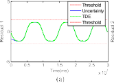
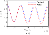
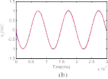
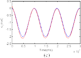
where the gains Kp 15I3 3, Kd 10I3 3, where In n rep- resents an identity matrix of dimension n n, are selected. The goal of the control system is to follow the desired tra- jectory xd [x1d, x2d, x3d]T with x1d cos(t/5π) 1, x2d cos(t/5π π/2) and x3d sin(t/5π π/2) 1 as shown in Fig. 3 (dashed blue line). When the robot in normal operation, φ(x1, x2, u) 0, TDE is the uncertainty estimation, HTDE (q, q,τ ). Fig. 1 shows the uncertainty estimation based on TDE. From this figure, we can see that the TDE technique gives a good capability to estimate an unknown non- linear function. For this reason, it is used as the residual to detect and isolate the faults. Then, from (30), the thresholds are selected as shown in Fig. 1 (dashed red line).
To verify the capability of the proposed TDE-based FD scheme for fault detection, isolation, and estimation, two kind of explicit faults are generated: 1) actuator bias faults and
part loss of effectiveness. First, an arbitrary abrupt fault


8 IEEE TRANSACTIONS ON CYBERNETICS


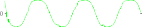
Fig. 1. Residuals of a healthy system and the selection thresholds.
(a) Residual 1. (b) Residual 2. (c) Residual 3.
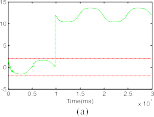
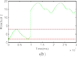
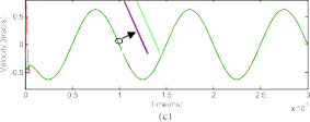
Fig. 2. Desired trajectories and joint angles of the robot manipulator when the actuator fault δτ1 occurs. (a) Joint 1. (b) Joint 2. (c) Joint 3.
=
≤
=
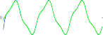
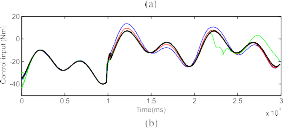
δτ1 [12(10 s), 0, 0]T is generated. It means that we sup- ply a bias fault in the first actuator with the magnitude 12 Nm at the time t 10 s. The angle trajectories when the robot in normal operation (t 10 s) and when the occurrence of fault δτ1 (t > 10 s) are shown in Fig. 2. Two obser- vations can be drawn from this figure: 1) under the effect of the fault δτ1, the tracking performance is reduced signif- icantly, and 2) the CTC controller do not compensate for the uncertainties in normal operation and both uncertainties and faults when the fault occurs; consequently, the track- ing performance of the system is very low (as shown in Tables I and II). The response of the residuals under the effect of the given fault is illustrated in Fig. 3. We can see that only the first residual overshoots the corresponding selected threshold, which indicates that the fault has been occurring in the first actuator. Therefore, it can be concluded that the fault is correctly detected and isolated. Then, we
supply an another complex fault δτ2 = [0, 20q2 + 15q˙2 +
Fig. 3. Response of the residuals of a faulty system under the effect of fault
δτ1. (a) Residual 1. (b) Residual 2. (c) Residual 3.
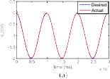
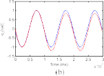
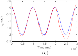
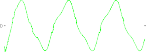
Fig. 4. Desired trajectories and joint angles of the robot manipulator when an actuator fault δτ2 occurs. (a) Joint 1. (b) Joint 2. (c) Joint 3.
at 10 s, and 75% partial loss fault in the third actuator at 20 s. Under the effects of fault δτ2, the tracking performance under CTC is much reduced as shown in Fig. 4. The correspond- ing responses of the three residuals are shown in Fig. 5. From Fig. 5, we can see that the second and third residuals overshoot the corresponding thresholds. Thus, we can conclude that the fault has been detected and isolated successfully.
Comparison Between BD and SOED for Velocity and Acceleration Estimation
=
=
In this section, we compare the performance of the SOED with BD technique in terms of velocity and acceleration esti- mation. The parameter of BD is selected as L 10−3 (this value is selected as the sampling time) and the parameters of SOED are all set to λ 5. The velocity estimation using BD and SOED techniques are shown in Fig. 6. From this figure, it
25 cos(q ) (10 s), 0.75u (20 s) T
1 1
can be seen that the SOED technique give a better performance
1 3 ] ; it means we supply in the
1
1
second actuator a bias fault δτ22 = 20q2 + 15q˙2 + 25 cos(q1)
compared to the BD technique.


VAN et al.: FINITE TIME FTC FOR ROBOT MANIPULATORS USING TDE AND CONTINUOUS NFTSMC 9


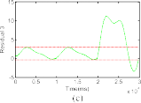
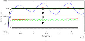
Fig. 5. Response of the residuals of a faulty system under the effect of fault
δτ2. (a) Residual 1. (b) Residual 2. (c) Residual 3.
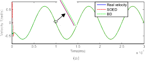
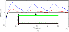
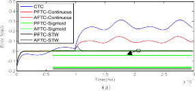
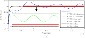
Fig. 7. Comparison in tracking error among CTC, PFTC-Continuous, AFTC-Continuous, PFTC-Sigmoid, AFTC-Sigmoid, PFTC-STW, and AFTC-STW when the actuator fault δτ1 occurs. (a) Error 1. (b) Error 2.
(c) Error 3.
TABLE I
COMPARISON IN ROOT MEAN SQUARE ERROR OF THE CTC, PFTC-CONTINUOUS, AFTC-CONTINUOUS, PFTC-SIGMOID, AFTC-SIGMOID, PFTC-STW, AND AFTC-STW WHEN
THE ACTUATOR FAULT δτ1 OCCURS


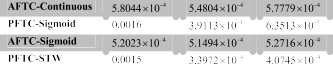

Fig. 6. Real and estimated velocities using BD and SOED techniques.
(a) Joint 1. (b) Joint 2. (c) Joint 3.
Comparison Between PFTC and AFTC Controllers Along With Chattering Elimination Techniques
In this section, the performance of the proposed PFTC and AFTC controllers along with chattering elimination techniques such as STW HOSM algorithm [as defined in (41)], contin- uous control law [as defined in (39)], and sigmoid approach [as defined in (40)] are compared. That means, we compare the performance of six developed controllers: 1) the pro- posed PFTC combined with STW HOSM (PFTC-STW); 2) the proposed AFTC combined with STW HOSM (AFTC-STW);
the proposed PFTC combined with continuous law (PFTC-Continuous); 4) the proposed AFTC combined with continuous law (AFTC-Continuous); 5) the proposed PFTC combined with sigmoid function approach (PFTC-Sigmoid); and 6) the proposed AFTC combined with sigmoid func- tion approach (AFTC-Sigmoid). These controllers are also compared with the conventional CTC controller. To easily compare the performance of PFTC and AFTC, the parameters of these controllers are chosen as the same value. In addi- tion, the parameters of the reduced chattering techniques are
10 IEEE TRANSACTIONS ON CYBERNETICS
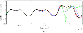
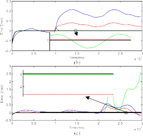
Fig. 8. Comparison in tracking error among CTC, PFTC-Continuous, AFTC-Continuous, PFTC-Sigmoid, AFTC-Sigmoid, PFTC-STW, and AFTC-STW when the actuator fault δτ2 occurs. (a) Error 1. (b) Error 2.
(c) Error 3.
fairly selected. The parameters of these controllers are selected
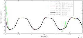
Fig. 9. Control efforts of the controllers (CTC, PFTC-Continuous, AFTC-Continuous, PFTC-Sigmoid, AFTC-Sigmoid, PFTC-STW, and AFTC-STW) when the system under the effect of actuator fault δτ2.
Joint 1. (b) Joint 2. (c) Joint 3.
TABLE II
COMPARISON IN ROOT MEAN SQUARE ERROR OF THE CTC, PFTC-CONTINUOUS, AFTC-CONTINUOUS, PFTC-SIGMOID, AFTC-SIGMOID, PFTC-STW, AND AFTC-STW WHEN
THE ACTUATOR FAULT δτ2 OCCURS
= = = =
as l 9, p 7, ϕ 1.5, σ1 diag(0.8, 0.8, 0.8), and


+ = =
= =
= = =
σ2 diag(1, 1, 1) for NFTSMC, k1 k2 7 for continu- ous law approach [defined in (39)], K1 5 and K2 6 for supper-twisting HOSM approach, and ρ η 6, b 1000 for the sigmoid function approach. The tracking errors of those controllers for the robot system under the faults δτ1 and δτ2 are shown in Figs. 7 and 8, respectively. For easy in compar-
ison, the root mean square error of those controllers for the


robot system under the faults δτ1 and δτ2 are also shown in
Tables I and II, respectively. From these figures and tables, two important observations can be given to verify the effectiveness of the proposed algorithm.
With the use of TDE for FD, the proposed AFTC has a much better performance compared to the PFTC in both fault-free and fault operation; for example: the per- formance of the AFTC-Continuous is better than the PFTC-Continuous, the AFTC-Sigmoid is better than the PFTC-Sigmoid, and the AFTC-STW is better than the PFTC-STW.
The use of STW HOSM gives a better performance compared to the used of continuous law and sigmoid approach; for example: the performance of PFTC-STW is better than PFTC-Continuous and PFTC-Sigmoid, and the AFTC-STW is better than that of AFTC-Continuous and AFTC-Sigmoid. The smooth control efforts of these
controllers for the system under the fault δτ2 are shown
in Fig. 9.
Comparison Between the Proposed NFTSMC and NTSMC and FTSMC
In this section, we compare the performance of AFTC based on the uses of the proposed NFTSMC, the NTSMC [the slid- ing surface is selected as in (10b)] [47] and the FTSMC [the sliding surface is selected as in (11)] [49]. The STW HOSM algorithm is employed to reduce the chattering. The tracking errors of these controllers for the robot system when the fault δτ1 occurred are shown in Fig. 10.
VAN et al.: FINITE TIME FTC FOR ROBOT MANIPULATORS USING TDE AND CONTINUOUS NFTSMC 11
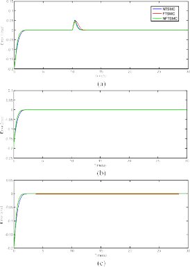
Fig. 10. Comparison in tracking error among NTSMC, FTSMC, and NFTSMC. (a) Error 1. (b) Error 2. (c) Error 3.
From Fig. 10, it is obvious to see that all the controllers provided a fast finite time convergence. However, the FTSMC and NFTSMC have a quite similar convergence but have a faster convergence compared to the NTSMC. However, as aforementioned analysis in Section III, the FTSMC may meet a singularity problem during operation. Thus, the NFTSMC would be a good choice to design a fast finite time FTC.
CONCLUSION